Design Resources Server

	Analysis of Data from Designed Experiments
	Resolvable Block Design

IASRI

Home

<<Back

Analysis Using SAS

Analysis Using SPSS

Main Procedure is:

Start →All Programs → SPSS for Windows → SPSS 15.0/ SPSS13.0/ SPSS10.0 (based on the version available on your machine) → Enter data in Data Editor → Analyze → GLM → Univariate → syield → [puts syield under Dependent list: ] → blk → [put blk under Fixed Factor(s): ] trt → [put trt under Fixed Factor(s):] Continue → Model... [Opens Model dialogue box] → Custom → Build Term(s) → Main effects → [puts rep blk, trt under Model: ] → Paste → It comes in Syntax mode, then define model as rep blk(rep) trt → Run all.

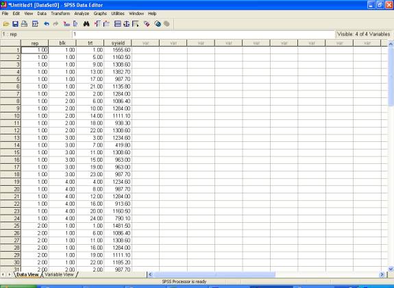
For performing analysis, input the data in the following format. Here the strain codes are termed as treatments trt, Replication as rep, block as blk and seed yield as syield. (It may, however, be noted that one can retain the same name or can code in any other fashion).

Following are the brief description of the steps along with screen shots.

· Open Data editor: Start → All Programs → SPSS for Windows → SPSS 15.0/ SPSS13.0/ SPSS10.0.

· Enter data in SPSS Data Editor. There are two views in SPSS Data Editor. In variable view, one can define the name of variables and variable types string or numeric and data view gives the spreadsheet in which data pertaining to variables may be entered in respective columns. In the present case, we enter data in numeric format

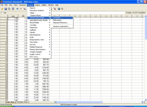
· Once the data entry is complete, Choose Analyze from the Menu Bar. Now select
Analyze → General linear Model → Univariate

· This selection displays the following screen

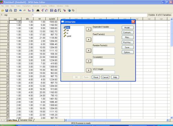
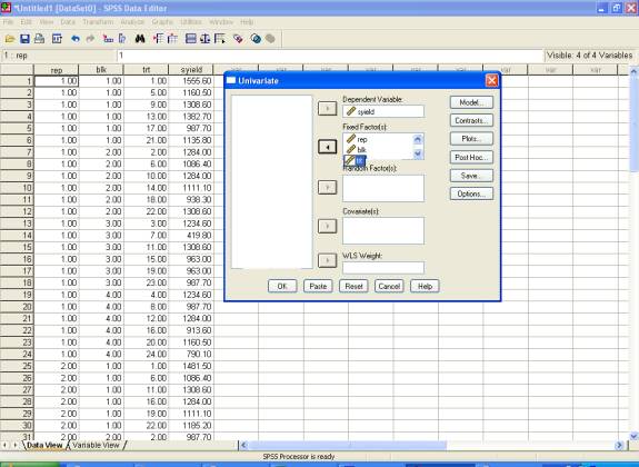
· Select syield and send it to the Dependent Variable box; blk and trt may be selected for Fixed
Factor(s) box. After doing these the dialog box should be like this

· Click Continue to return back to the Univariate dialog box, then click paste to get the commands in
syntax editor. Now define model as per design adopted to analyze the data. Here it is
/Design = rep blk(rep) trt.

       For identification of the treatments that gave significantly higher yield than the best performing check, one
       can write all possible elementary contrasts between checks, i.e. 20, 21 and 23 and identify the best
       performing check. This can be identified using the contrast estimates.
      /Lmatrix '20 vs 21' trt 0 0 0 0 0 0 0 0 0 0 0 0 0 0 0 0 0 0 0 1 -1 0 0 0;
      /Lmatrix '20 vs 23' trt 0 0 0 0 0 0 0 0 0 0 0 0 0 0 0 0 0 0 0 1 0 0 -1 0;
      /Lmatrix '21 vs 23' trt 0 0 0 0 0 0 0 0 0 0 0 0 0 0 0 0 0 0 0 0 1 0 -1 0;

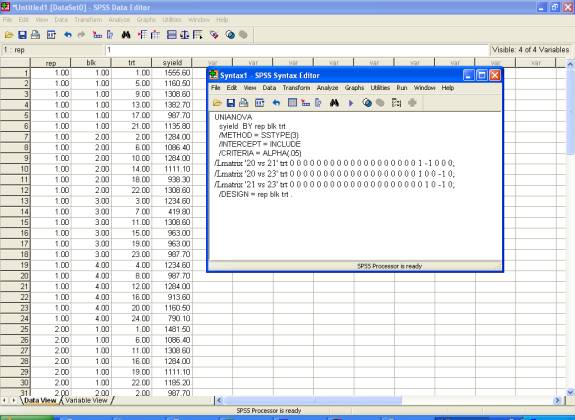
· Click Run → All.

The following syntax may be used after creating the data file to get the output.

UNIANOVA

syield BY rep blk trt

/METHOD = SSTYPE(3)

/INTERCEPT = INCLUDE

/CRITERIA = ALPHA(.05)

/Lmatrix '20 vs 21' trt 0 0 0 0 0 0 0 0 0 0 0 0 0 0 0 0 0 0 0 1 -1 0 0 0;

/Lmatrix '20 vs 23' trt 0 0 0 0 0 0 0 0 0 0 0 0 0 0 0 0 0 0 0 1 0 0 -1 0;

/Lmatrix '21 vs 23' trt 0 0 0 0 0 0 0 0 0 0 0 0 0 0 0 0 0 0 0 0 1 0 -1 0;

/DESIGN =rep blk(rep) trt .

One can easily see that treatment 21 is the best performing check. Now make 21 elementary contrasts for comparing best performing check (21) with each of the new strains (1, 2, 3, 4, 5, 6, 7, 8, 9, 10, 11, 12, 13, 14, 15, 16, 17, 18, 19, 22, 24). This will be helpful for identifying the strains that perform significantly better than the best performing check. The contrasts may be written as above or as in Incomplete block designs.

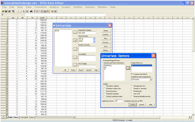
Alternatively, all possible pair wise treatment comparisons can be performed using the Button Options on the dialogue box. A click on Button Options, gives the option for estimated marginal means and display means for. From the left hand box, take the effect treatment in the Display means for. Then check the box Compare main effects and then there are 3 options for confidence interval adjustment viz. LSD(none), Bonferrnoni and Sidak. Any one of these 3 options can be selected. Default option is LSD(None). A screen shot for these options is