Data Input:

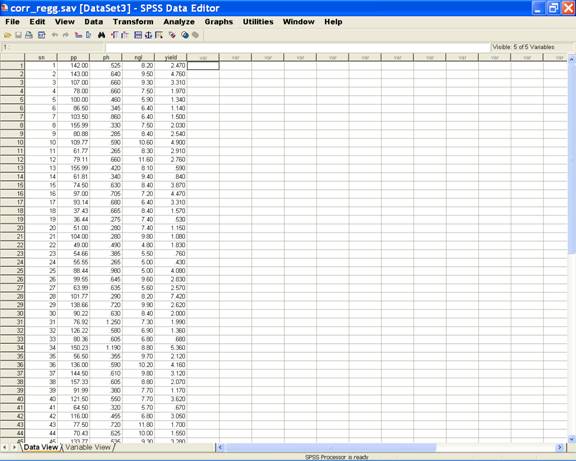
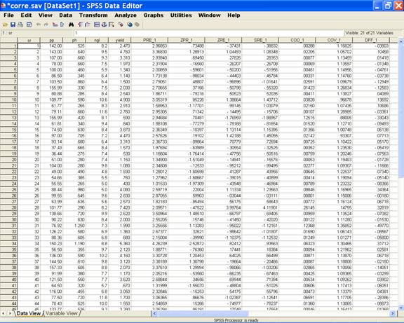
For performing analysis, input the data in the following format. 

{Here serial number is termed as SN, plant population as PP, average plant height as PH, average number of green leaves as (NGL) and yield as YLD. It may, however, be noted that one can retain the same name or can code in any other fashion}.

 Following are the brief description of the steps along with screen shots.

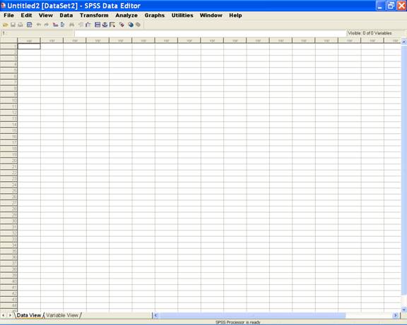
·         Open Data editor: Start → All Programs → SPSS for Windows → SPSS 15.0/ SPSS13.0/  SPSS10.0

·         Enter data in SPSS Data Editor. There are two views in SPSS Data Editor. In variable view, one can define the name of variables and variable types string or numeric and data view gives the spreadsheet in which data pertaining to variables may be entered in respective columns. In the present case, we enter data in numeric format.

·      Obtain correlation coefficient between each pair of the variables PP, PH, NGL and yield by using the following steps

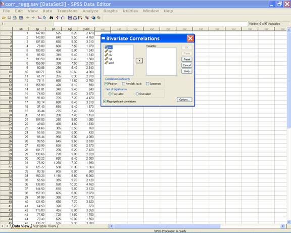
            Once the data entry is complete, Choose Analyze from the Menu Bar. Now select   Analyze → Correlate → Bivariate. 

·         This selection displays the following screen.

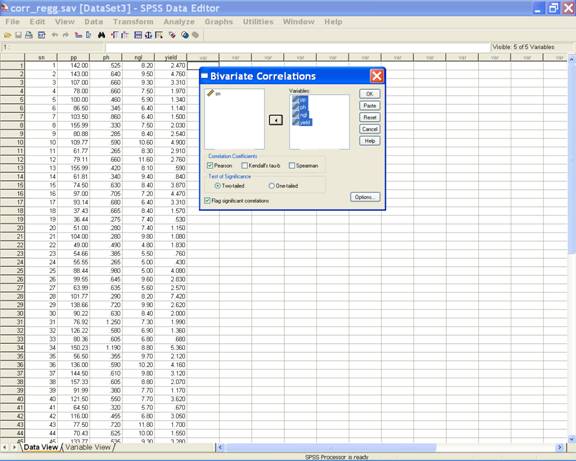
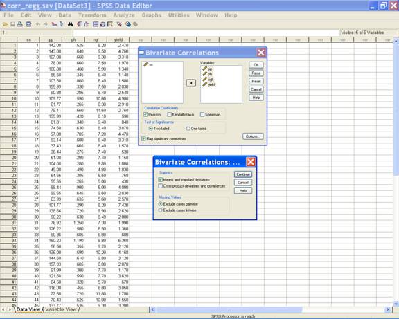
·         In the Bivariate Correlations dialog box select the biometrical characters pp, ph, ngl and yield and send them to the Variables box. This displays the following screen.

·         Select Options in the Bivariate Correlations dialog box. Under the Statistics option check the Means and standard deviations check box. This selection displays the following screen.

·      Click Continue to return to the Bivariate Correlations dialog box.

·      Click OK

 Obtain partial correlation between NGL and yield after removing the linear effect of PP and PH by using the following steps.

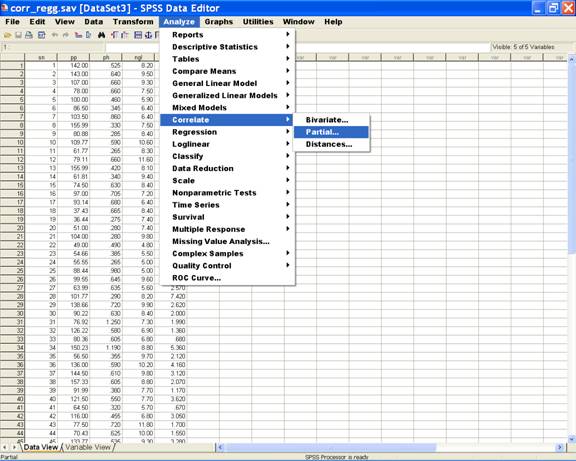
·  Choose Analyze from the Menu Bar. Now select   Analyze → Correlate → Partial. 

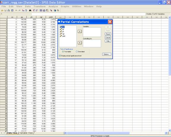
·         This selection displays the following screen.

·         In the Partial Correlations dialog box select yield and ngl and send them to the Variables box and send pp and ph to the Controlling for box. This displays the following screen.

·         Select Options in the Partial Correlations dialog box. Under the Statistics option check the Means and standard deviations check box. This selection displays the following screen.

·      Click Continue to return to the Partial Correlations dialog box.

·      Click OK.

  Obtain the scatter plot using the following steps.

·         Choose Graphs from the Menu Bar. Now select   Graphs → Interactive→ Scatterplot.

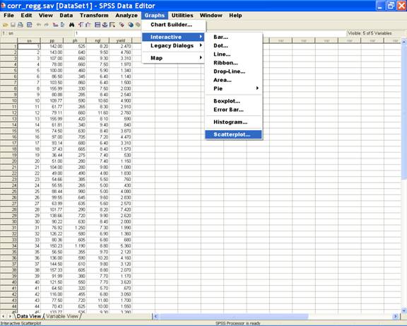
·         This selection displays the following screen.

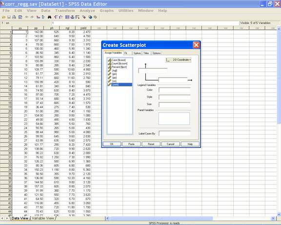
·         In the Assign Variables tab put pp in the vertical axis and yield in the horizontal axis. This selection displays the following screen.

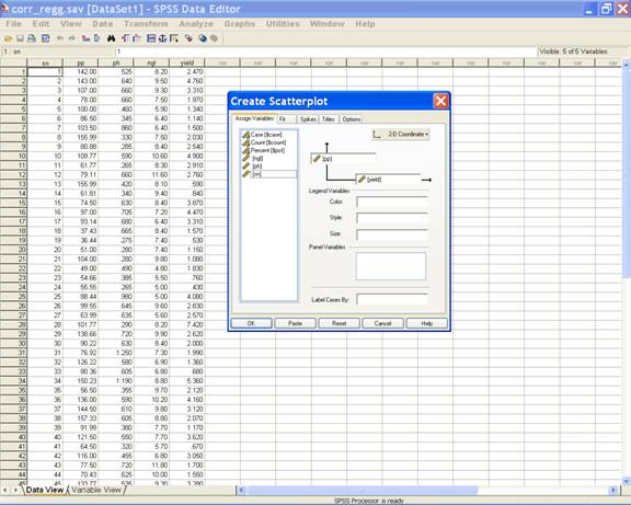
·      Click OK

  Fit a multiple linear regression equation by taking yield as dependent variable and biometrical characters as explanatory variables. By using the following steps:

·      Choose Analyze from the Menu Bar. Now select   Analyze → Regression → Linear.

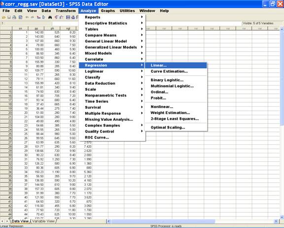
·      This selection displays the following screen

.

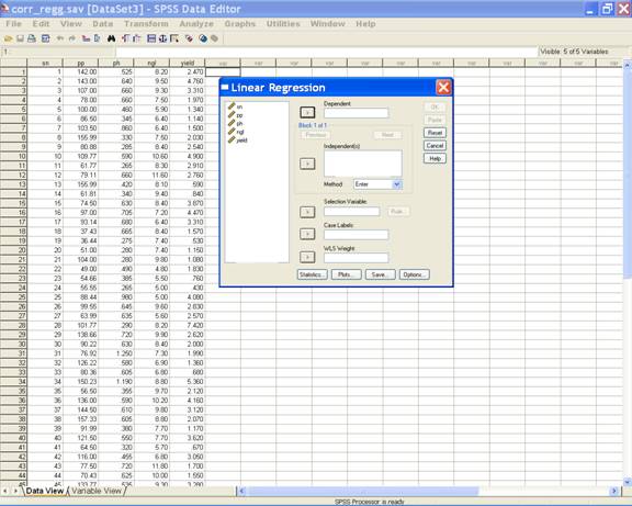
·      In the Linear Regression dialog box select yield and send it to the Dependent Variable box; select and send pp, ph and ngl to the independent(s) variable box. This displays the following screen.

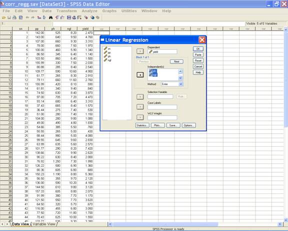
·      For the Durbin-Watson statistics click Statistics on the Linear Regression dialog box. In the Linear Regression: Statistics dialog box check the Durbin-Watson check box under Residuals and other options as required. This displays the following screen.

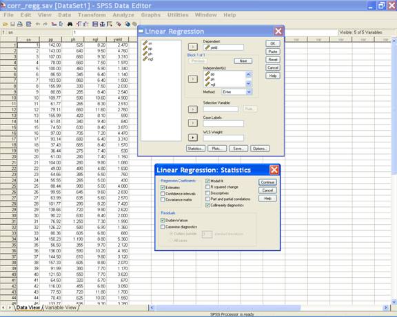
·      Click Continue to return to the Linear Regression dialog box.

·Click Save in the Linear Regression dialog box. In the Linear Regression: Save dialog box check the desired options under Predicted Values, Residuals, Distances and Influence Statistics. This selection displays the following screen.

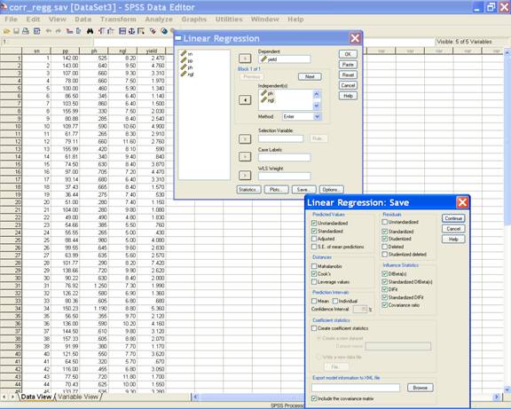
·      Click Continue to return to the Linear Regression dialog box.

A regression model without intercept can be fitted by using the following procedure

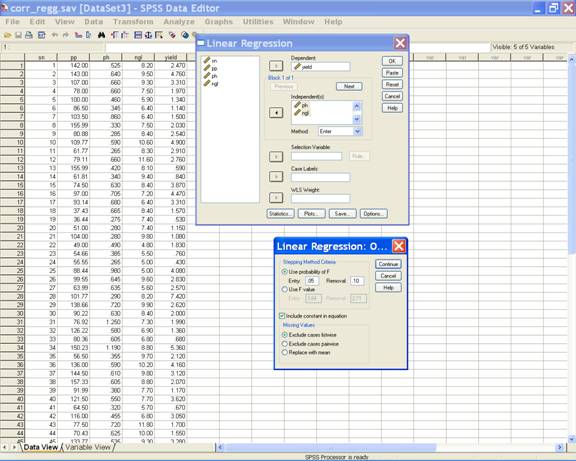
·      In the Linear Regression dialog box Click Options. This selection displays the following screen.

·      For the regression model without intercept uncheck the include constant in equation option. This selection displays the following screen.

·      Click Continue to return to the Linear Regression dialog box.

·      Click OK.

·      Some output results for the regression analysis are produced in the SPSS Data editor. Which are as follows:

·      To answer all the questions 1 to 8, the following syntax may be used after creating the data file.

CORRELATIONS

  /VARIABLES=yield pp ph ngl

  /PRINT=TWOTAIL NOSIG

  /STATISTICS DESCRIPTIVES

  /MISSING=PAIRWISE .

PARTIAL CORR

  /VARIABLES= yield ngl BY pp ph

  /SIGNIFICANCE=TWOTAIL

  /STATISTICS=DESCRIPTIVES

  /MISSING=LISTWISE .

IGRAPH /VIEWNAME='Scatterplot' /X1 = VAR(yield) TYPE = SCALE /Y = VAR(pp)

  TYPE = SCALE /COORDINATE = VERTICAL  /X1LENGTH=3.0 /YLENGTH=3.0

 /X2LENGTH=3.0 /CHARTLOOK='NONE' /SCATTER COINCIDENT = NONE.

EXE.

REGRESSION

  /MISSING LISTWISE

  /STATISTICS COEFF OUTS R ANOVA COLLIN TOL

  /CRITERIA=PIN(.05) POUT(.10)

  /NOORIGIN

  /DEPENDENT yield

  /METHOD=ENTER pp ph ngl

  /RESIDUALS DURBIN

  /SAVE PRED ZPRED COOK ZRESID SRESID DFBETA SDBETA DFFIT SDFIT COVRATIO .