Analysis Using SPSS

 Main Procedure is:  

Start →All Programs → SPSS for Windows → SPSS 15.0/ SPSS13.0/ SPSS10.0 (based on the version available on your machine) → Enter data in Data Editor → Analyze → GLM → Univariate  → yield → [puts yield under Dependent list: ] → rep → [put rep under Fixed Factor(s): ]   ms → [put ms under Fixed Factor(s):]  mt → [put mt under Fixed Factor(s):]  Continue → Model... [Opens Model dialogue box] → Custom → Build Term(s) → Main effects  →[puts rep, ms, mt under Model: ] Interaction→rep → var → spt  → [puts rep*ms and ms*mt  under Model:] → Run All.

Data Input:

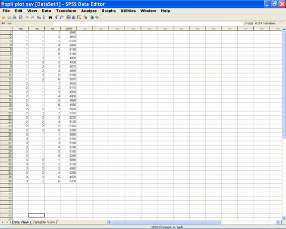
For performing analysis, input the data in the following format. {Here one can call the replication as rep, main-plot treatments as ms (method of sowing) and sub-plot treatments as mt (manorial treatment). (It may, however, be noted that one can retain the same name or can code in any other fashion).

 Following are the brief description of the steps along with screen shots.

·         Open Data editor: Start → All Programs → SPSS for Windows → SPSS 15.0/ SPSS13.0/  SPSS10.0  

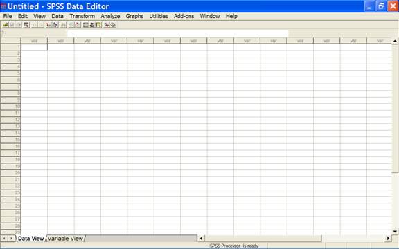
·         Enter data in SPSS Data Editor. There are two views in SPSS Data Editor. In variable view, one can define the name of variables and variable types string or numeric and data view gives the spreadsheet in which data pertaining to variables may be entered in respective columns. In the present case, entered data is in numeric format.

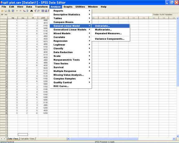
·         Once the data entry is complete, Choose Analyze from the Menu Bar. Now select Analyze → General linear Model → Univariate.  

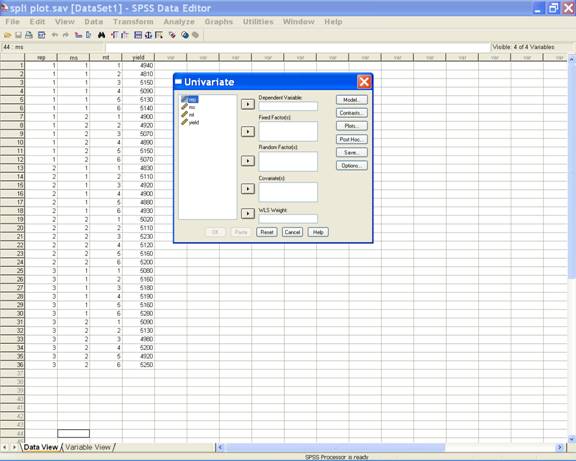
• This selection displays the following screen:  

• Select yield and send it to the Dependent Variable rep, ms and mt may be selected for Fixed Factor(s) box. This selection displays the following screen:

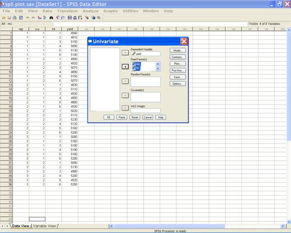
• For the Interactions select Model in the Univariate dialog box i.e. → Model... [Opens Model dialogue box] → Interaction→ rep → ms → [puts rep*ms under Model:].Similarly ms*mt can also be put under the model.

This selection displays the following screen.

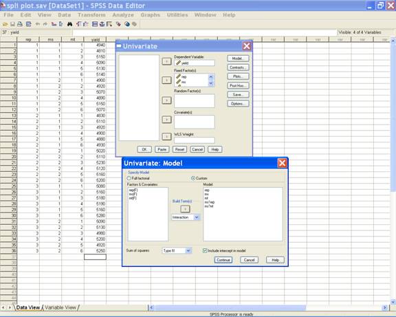
·         Click  Continue to return to the Univariate dialog box .

Syntax for testing mainplot with error(a).

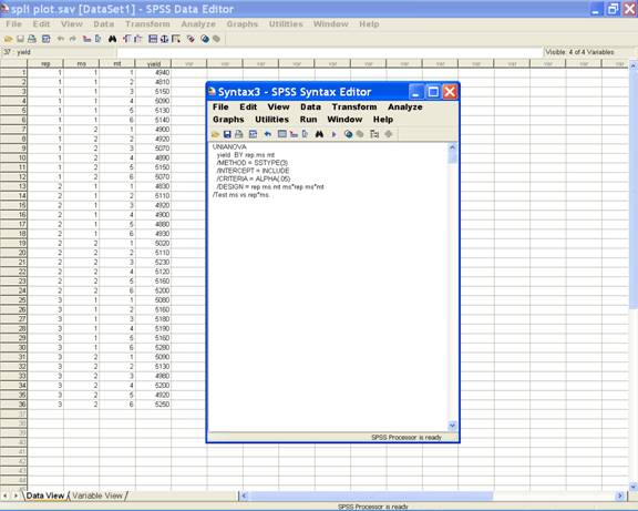
·         Click Run → All.

To perform the analysis, the following syntax may be used after creating the data file.

UNIANOVA

  YIELD  BY REP MS MT

  /METHOD = SSTYPE(3)

  /INTERCEPT = INCLUDE

  /CRITERIA = ALPHA(.05)

  /DESIGN = REP MS MT MS*REP MS*MT

/TEST MS VS REP*MS.

We could not find the syntax for pairwise comparisons by selecting the appropriate error term. For making all possible pairwise comparisons, one may, however, compute only the means from the software and compute the minimum significant differences using the given formulae on the click of mouse.