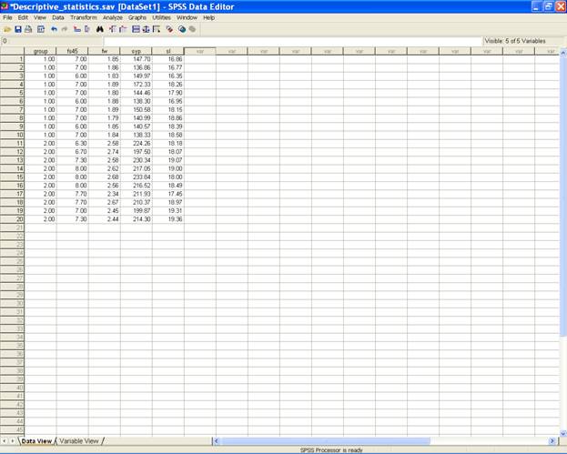
For performing analysis, input the data in the following format. 

{Here Number of fruit (45 days) is termed as nfs45, Fruit weight (kg) is termed as fw, seed yield/plant (g) is termed as syp and Seedling length (cm) is termed as sl. It may, however, be noted that one can retain the same name or can code in any other fashion}.

 Following are the brief description of the steps along with screen shots. 

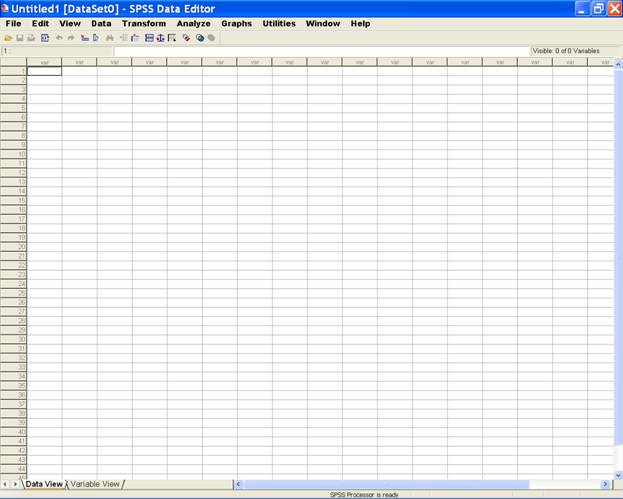
• Open Data editor: Start → All Programs → SPSS for Windows → SPSS 15.0/ SPSS13.0/ SPSS10.0

•  Enter data in SPSS Data Editor. There are two views in SPSS Data Editor. In variable view, one can define the name of variables and variable types such as string or numeric and data view gives the spreadsheet in which data pertaining to variables may be entered in respective columns. In the present case, we enter data in numeric format.

        To answer the questions

         1. Obtain mean, standard deviation, minimum and maximum values of all the characters.

         3. Obtain mean, median, coefficient of skewness, coefficient of kurtosis of all the characters.

         8. Create a stem and leaf plot and box plot for all the characters.

the following steps may be used.

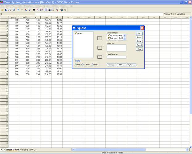
•   Choose Analyze from the Menu Bar. Now select Analyze → Descriptive statistics → Explore…

•   This selection displays the following screen.

• Select fs45, fw, syp and sl and send it to the Dependent List box. Select the Both( Default Option) tab in the Display option.

• This selection displays the following screen.

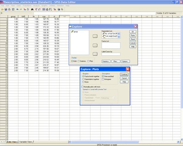
• To plot the stem and leaf plot and box plot click on the Plot… tab in the explore dialog box and select the options for the respective plots.

• This selection displays the following screen.

• Click on Continue to return to the Explore dialog box.

• Click on OK to get the output.

• To answer the questions 1, 3 and 8 the following syntax may be used.

EXAMINE

  VARIABLES=fs45 fw syp sl

  /PLOT BOXPLOT STEMLEAF

  /COMPARE GROUP

  /STATISTICS DESCRIPTIVES

  /CINTERVAL 95

  /MISSING LISTWISE

  /NOTOTAL.

  Alternative Method 1: to answer the questions

                1. Obtain mean, standard deviation, minimum and maximum values of all the characters.

                3. Obtain mean, median, coefficient of skewness, coefficient of kurtosis of all the characters.

                6. Prepare a discrete frequency table for all the characters for the above data on group.

  the following steps may be used.

•   Choose Analyze from the Menu Bar. Now select Analyze → Descriptive Statistics → Frequencies…

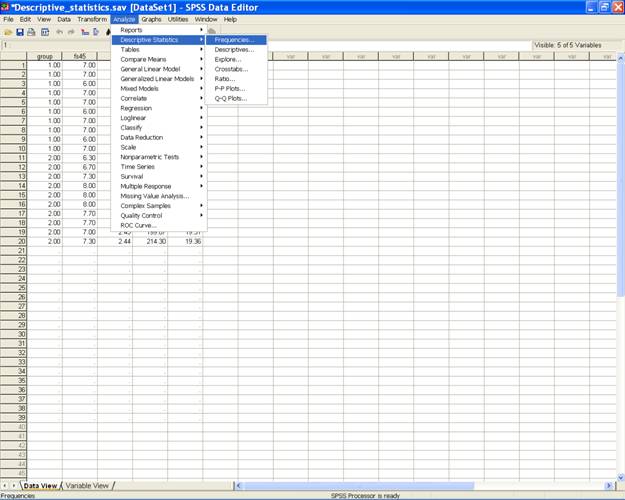
•      This selection displays the following screen.

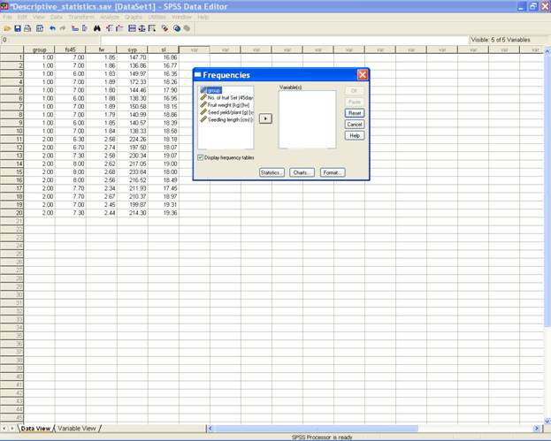
• Select fs45, fw, syp and sl and send it to the variable box.

• Click on the Statistics… tab to get the Frequencies: Statistics dialog box. Select the desired options (Mean, Std. Deviation, Minimum, Maximum, Skewness and Kurtosis) required for analysis.

•  To answer the question

       6.  Prepare a discrete frequency table for all the characters for the above data on group.

 put a check for the Display frequency tables on the Frequencies dialog box.

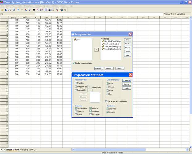
• Click on the Continue tab to return to the Frequencies dialog box.

• Click on OK to get the output.

                          For the Alternative Method 1: to answer the questions 1, 3 and 6 the following syntax may be used.

                     FREQUENCIES

                        VARIABLES=fs45 fw syp sl

                           /STATISTICS=STDDEV MINIMUM MAXIMUM MEAN SKEWNESS SESKEW KURTOSIS SEKURT

                           /ORDER=  ANALYSIS .

                 Alternative Method 2: to answer the questions

                   1.   Obtain mean, standard deviation, minimum and maximum values of all the characters.

                   3.  Obtain mean, median, coefficient of skewness, coefficient of kurtosis of all the characters.

the following steps may be used.

• Choose Analyze from the Menu Bar. Now select Analyze → Descriptive Statistics → Descriptives…

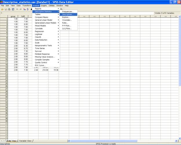
•  This selection displays the following screen.

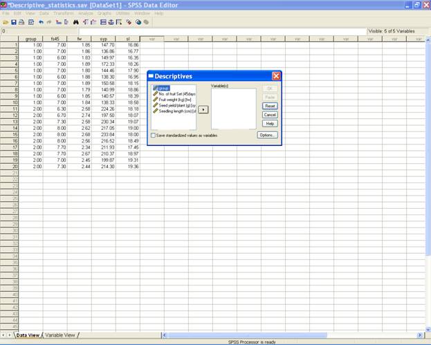
• Select fs45, fw, syp and sl and send it to the variable(s): box.

• This displays the following screen.

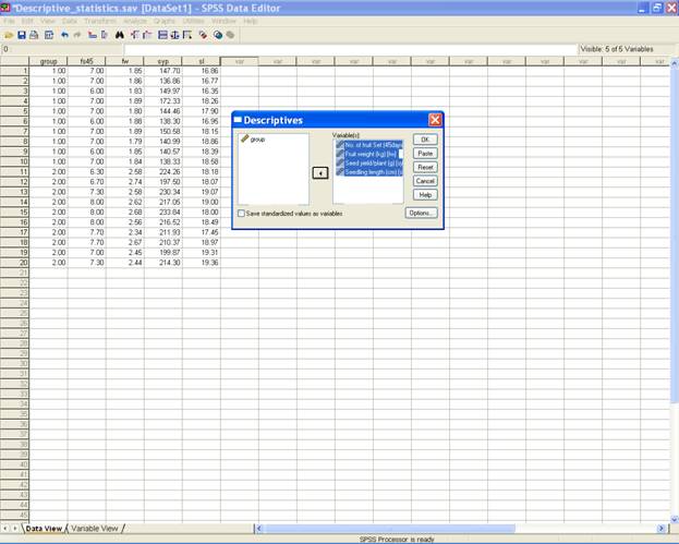
• Click on the Options… tab on the Descriptives dialog box. Select the required statistics (Mean, Std. Deviation, Minimum, Maximum, Skewness and Kurtosis) for analysis.

• This selection displays the following screen.

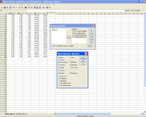
• Click on the Continue tab to return to the Descriptives dialog box.

• Click on OK to get the output.

 For the Alternative Method 2:  to answer the questions 1 and 3 the following syntax may be used.

DESCRIPTIVES

  VARIABLES=fs45 fw syp sl

  /STATISTICS=MEAN STDDEV MIN MAX KURTOSIS SKEWNESS .

             To answer the questions

          2.  Obtain mean, standard deviation, minimum and maximum values of all the characters for  

          4.  Obtain mean, median, coefficient of skewness, coefficient of kurtosis of all the characters for each of the group separately.

          5.   Test whether the data follows a normal distribution or not for all the characters? Do it separately for each of the two groups.

          9.   Create a stem and leaf plot and box plot for all the characters for each group separately.

              the following steps may be used.

•      Choose Analyze from the Menu Bar. Now select Analyze → Descriptive statistics → Explore…

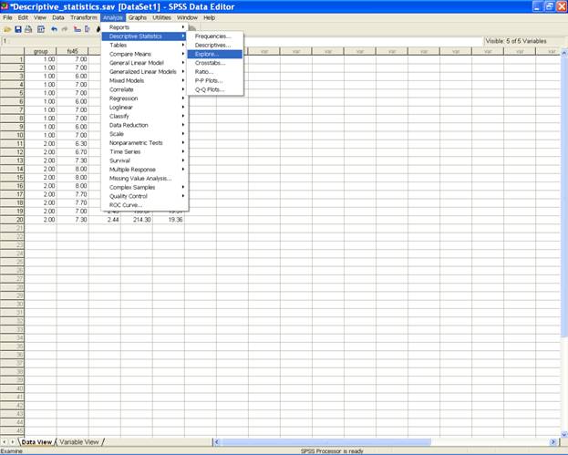
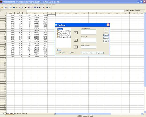
•      This selection displays the following screen.

• Select fs45, fw, syp and sl and send it to the Dependent List box. Select group and send it to the Factor List box.

• Select the Both option in the Display option.

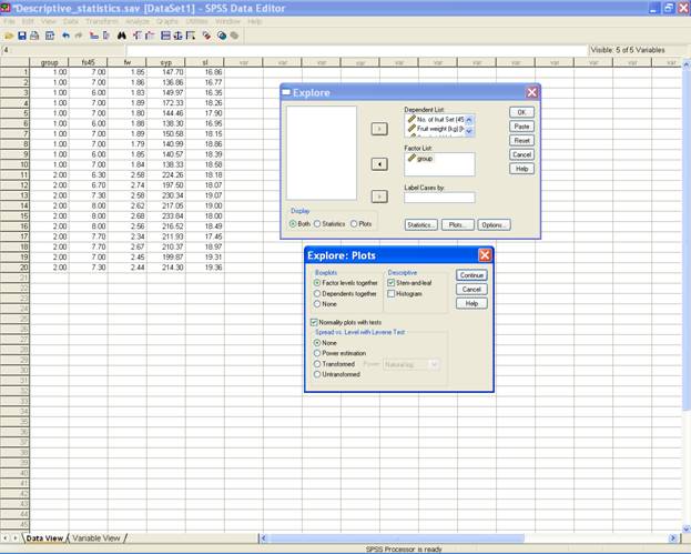
• To create a stem and leaf plot and box plot and to test whether the data follows normal distribution or not, click on the Plots… tab in the explore dialog box. Select the required options in the Explore: Plots dialog box.

• To test whether the data follows a normal distribution or not put a check against the option Normality plots with tests.

• This selection displays the following screen.

• Click on Continue to return to the explore dialog box.

• Click on OK to get the output.

 To answer the questions  2, 4, 5 and 9 the following syntax may be used.

EXAMINE

  VARIABLES=fs45 fw syp sl BY group

  /PLOT BOXPLOT STEMLEAF NPPLOT

  /COMPARE GROUP

  /STATISTICS DESCRIPTIVES

  /CINTERVAL 95

  /MISSING LISTWISE

  /NOTOTAL.

To answer question

7. To prepare 2-way frequency table between group and fruit set after 45 days the following steps may be used.

• Choose Analyze from the Menu Bar. Now select Analyze → Descriptive Statistics → Crosstabs…

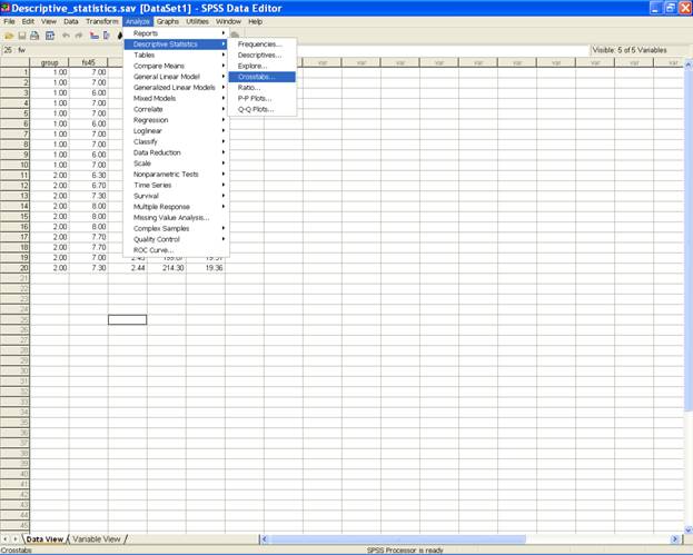
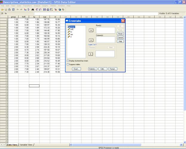
• This selection displays the following screen.

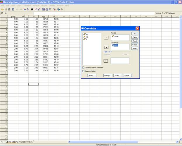
• Select the variable group and send it to the Row(s): box and fs45 to the Column(s): box.

• This selection would display the following screen.

• Click on OK to get the output

For question 7. To prepare 2-way frequency table between group and fruit set after 45 days the following syntax may be used.

CROSSTABS

  /TABLES=group  BY fs45

  /FORMAT= AVALUE TABLES

  /CELLS= COUNT

  /COUNT ROUND CELL .

To answer question

              10.   Make the grouped frequency distribution by dividing the data on seed yield per plant in 10 classes  135-145, 145-155, 155-165,165-175, 175-185, 185-195, 195-205, 205-215, 215-225, 225-235 with upper limits exclusively and their frequencies.

the following steps may be used.

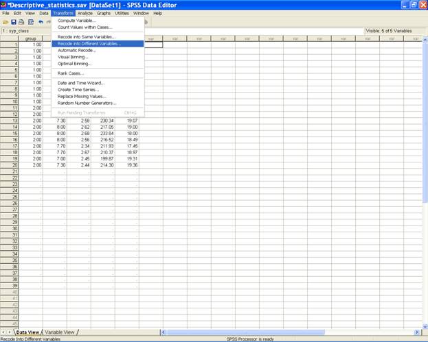
•     Choose Transform from the Menu Bar. Now select Transform → Recode into Different Variables…

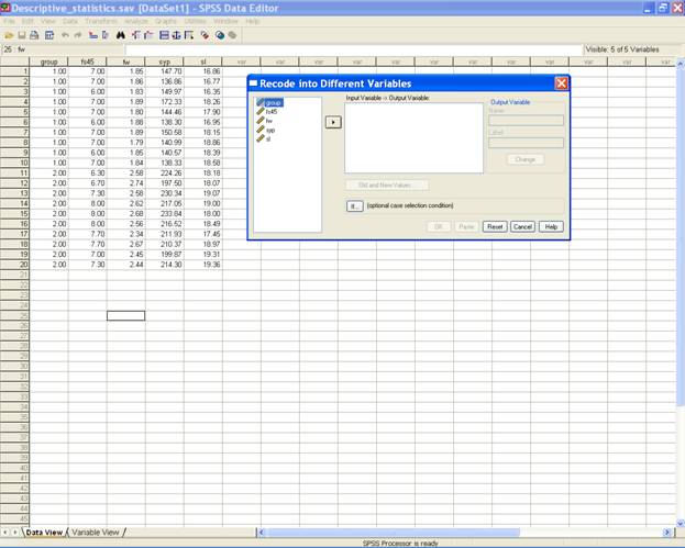
•        This selection displays the following screen.

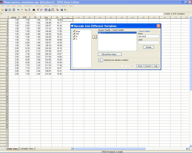
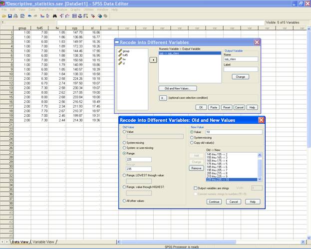
• Select the variable for which the frequency distribution is required( in our case it is syp) and send it to the Numeric Variable → Output Variables box.

• Define the Output Variable name and click on Change tab.

•  This selection displays the following screen.

• Click on the Old and New Values… tab.

• This selection displays the following screen.

• Define the range for the frequency distribution and give the name for the new value.

• Add this new value to the Old → New box.

• This selection displays the following screen.

• Click on Continue to return to the Recode into Different Variables… dialog box.

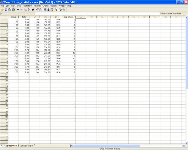
• Click on OK to get the output for the frequencies in the SPSS data editor as follows.

To answer question  10 the following syntax may be used.

RECODE

  syp

  (135 thru 145=1)  (145 thru 155=2)  (155 thru 165=3)  (165 thru 175=4)

 (175 thru 185=5)  (185 thru 195=6)  (195 thru 205=7)  (205 thru 215=8)

 (215 thru 225=9)  (225 thru 235=10)  INTO  syp_class .

EXECUTE .

                To answer the question

       11. To prepare a histogram for the grouped frequency distribution in question number 10 the following steps may be used.

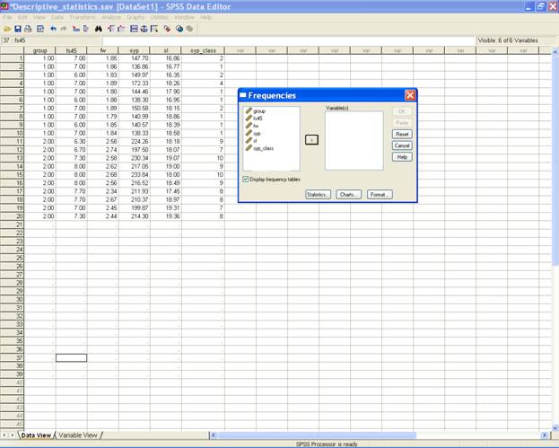
•       Choose Analyze from the Menu Bar. Now select Analyze → Descriptive Statistics → Frequencies…

•        This selection displays the following screen.

•       Select the variable syp and send it to the Variable(s): box.

•      Check the option for Display frequency tables to get the grouped frequency table.

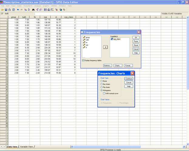
•        Click on Charts… tab and in the Frequencies: Chart dialog box and select the Chart type as Histograms.

•       This selection displays the following screen.

• Click on Continue to return to the Frequencies dialog box.

• Click on OK to get the output.

The following syntax may be used to prepare a histogram for the grouped frequency distribution in question number 10.

FREQUENCIES

  VARIABLES=syp_class

  /HISTOGRAM

  /ORDER=  ANALYSIS .

<<Back

      Analysis Using SAS                                           Analysis Using SPSS                                           

Home Descriptive Statistics  Tests of Significance Correlation and Regression Completely Randomised Design  RCB Design  

Incomplete Block Design  Resolvable Block Design  Augmented Design  Latin Square Design Factorial RCB Design  

Partially Confounded Design Factorial Experiment with Extra Treatments Split Plot Design Strip Plot Design 

Response Surface Design Cross Over Design  Analysis of Covariance Diagnostics and Remedial Measures 

Principal Component Analysis Cluster Analysis Groups of Experiments  Non-Linear Models  

Contact Us