| Design Resources Server |
|
||||
| IASRI | |||||
| Home |
Analysis Using SPSS
NOTE:
Description of Nonlinear Models and Percentage Forecast
Error The mathematical representation of the nonlinear models mentioned in the problem is as follows 1. Logistic model is given by X(t)=c/(1+b*exp(-a*t)) + e(t) , 2. Gompertz Model is represented by X(t) = c*exp(-b*exp(-a*t)) + e(t), 3.
Monomolecular model is given by X(t)
= c-(c-b)*exp(-a*t) +
e(t), where X(t) denotes the variable under study at time t, �a� denote the intrinsic growth rate, �c� the carrying capacity of the environment, b = [b-X(0)]/X(0) and X(0) is the value of X(t) at t = 0 and e(t) is the error term. In general the parameter �a� is the coefficient of external influence emanating from the outside system. One
Step Ahead Forecasting (OSAF) In OSAF method the last observation is not considered and the
model is fitted to the data set. The last value is predicted
from the model and is compared with the actual value. The
percentage forecast error (PCFE) is defined as
PCFE =
where
X(t) is the observed value and
Refrence: Draper,N.R.
and Smith,H.(2005). Applied regression analysis, 3rd
ed. John Wiley and Sons, Seber,G.A.F
and Wild,C.J.(2003). Nonlinear regression. John-Wiley &
sons. Das,P.K.(1995).
Nonlinear models for studying acreage, production and
productivity of wheat in Ratkowsky,
D.A. (1990). Handbook of nonlinear regression models. Marcel
Dekker, Ronald,G.A.(1987).
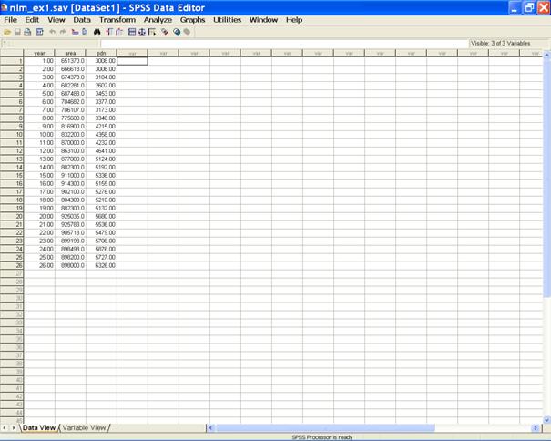
Nonlinear statistical models. John Wiley and sons, For Fitting nonlinear models input the data in the following format. {Here year is considered as independent variable and area and production( pdn) are considered as dependent variables. It may, however, be noted that one can retain the same name or can code in any other fashion.} Following are the brief description of the steps along with screen shots. � Enter data in SPSS Data Editor. There are two views in SPSS Data Editor. In variable view, one can define the name of variables and variable type string or numeric and data view gives the spreadsheet in which data pertaining to variables may be entered in respective columns. In the present case, we enter data in numeric format.
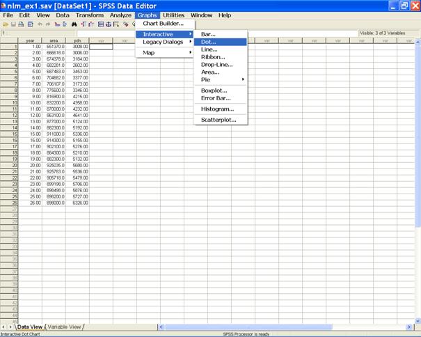
Steps to draw scatter plot for area versus year. �
Choose Analyze from the Menu Bar. Now select Graphs
→ Interactive → Dot�
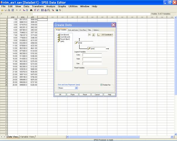
� In the Create Dots dialog box select the variable area for the y-axis and year for the x-axis.
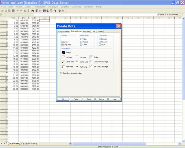
� Select the tab Dots and Lines. In the Display option select Lines and Drop lines. � This displays the following screen.
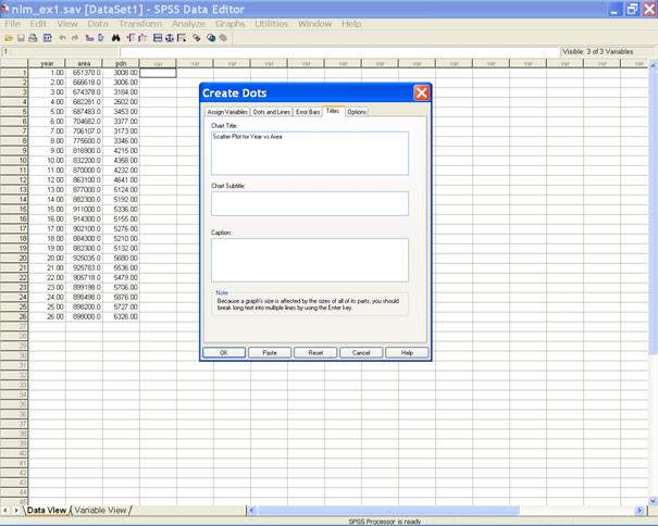
� Click on the Titles tab to define the title for the graph.
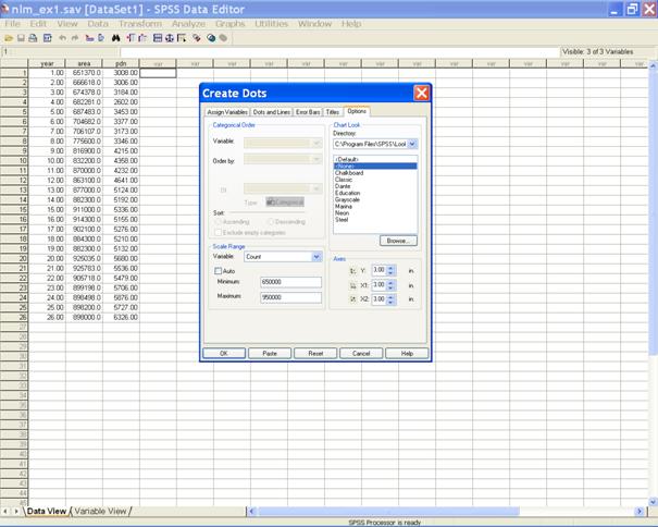
� Select the Options tab. In the Create Dots dialog box define the Minimum and the Maximum values for the Scale range
� Click on OK to get the scater plot as output. � Similarly the scater plot for �Year vs Production' and �Year vs ' Productivity' may be obtained. The following syntax may be used after creating the data file to create the scatter plot. /* scatter plot for area versus year*/ IGRAPH
/VIEWNAME='Dot Chart' /X1 = VAR(year) TYPE = SCALE /Y =
VAR(area) TYPE =
SCALE /COORDINATE = VERTICAL
/TITLE='Scater Plot for Year vs Area' /X1LENGTH=7.0
/YLENGTH=7.0 /X2LENGTH=3.0 /CHARTLOOK='NONE' /SCALERANGE =
VAR(area) MIN=650000.000000 MAX=950000.000000 /LINE(MEAN)
KEY=ON STYLE = DOTLINE DROPLINE
= ON INTERPOLATE = STRAIGHT BREAK = MISSING. EXE. /* scatter plot for production versus year*/ IGRAPH
/VIEWNAME='Dot Chart' /X1 = VAR(year) TYPE = SCALE /Y =
VAR(pdn) TYPE =
SCALE /COORDINATE = VERTICAL
/TITLE='Scater Plot for Year vs pdn' /X1LENGTH=7.0
/YLENGTH=7.0 /X2LENGTH=3.0 /CHARTLOOK='NONE' /LINE(MEAN)
KEY=ON STYLE =
DOTLINE DROPLINE = ON INTERPOLATE = STRAIGHT BREAK =
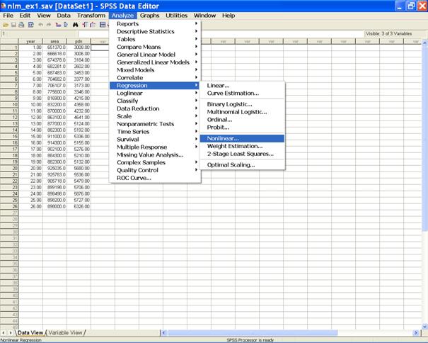
MISSING. EXE. To fit the nonlinear regression model follow the following steps. � Choose Analyze from the Menu Bar. Now select Analyze→ Regression → Nonlinear�
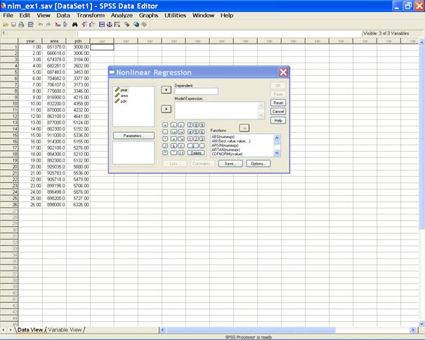
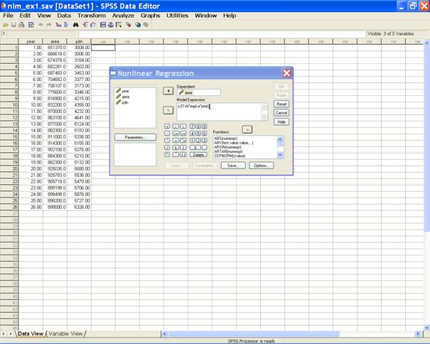
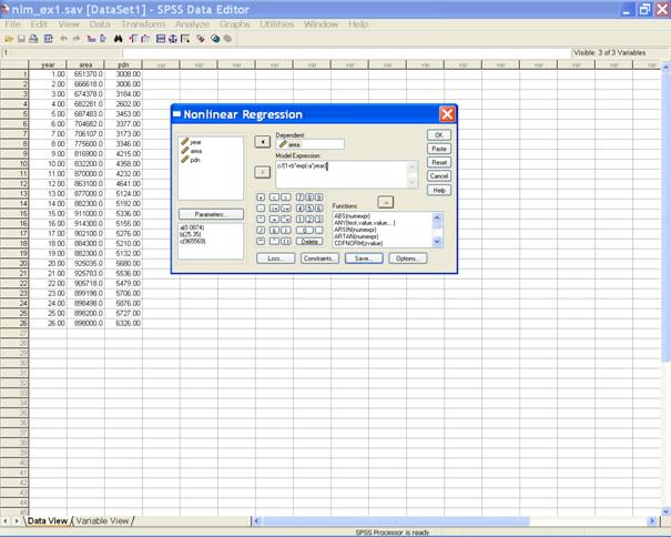
� The following dialog box appears.
� Send area to the Dependent variable box. In the Model Expression: box define the model expression.
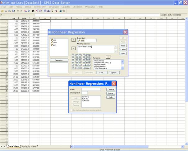
� Click on Parameters tab to get the Nonlinear Regression: Parameters dialog box. � Here in the Name option define the name of the parameter and assign the starting value of the defined parameter and click on Add tab. Similarly we may assign the remaining parameters of the model.
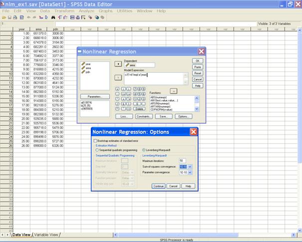
� Click on Continue to return to the Nonlinear Regression dialog box. � Click on the options tab to get the following window. NOTE :
The methods for obtaining initial parameter values
for Logistic, Gompertz and Monomolecular model are same.
Logistic model is given by the following equation X(t) = c/(1+b*exp(-a*t)), where b= [c-X(0)]/X(0) and X(0) is the value X(t) at t=0. The value of �c� is obtained from the plot X(t) versus t through visual examination and denote the value of �c� as �c0�, then value of b as b0 = [c0-X(0)]/X(0) Rearranging eq. (1) we get Z0 = ln{[c0/X(t) -1]/b0} = - At This is a linear equation in parameter A. Now we can apply linear regression to the eq. 2, i.e. Z0 on t and obtain the estimate of A as a0. Hence, we have obtained the initial values of the three parameters a, b and c as a0, b0 and c0 respectively. Draper,N.R. and Smith,H.(2005). Applied regression analysis, 3rd ed. John Wiley and Sons, New York. Seber,G.A.F
and Wild,C.J.(2003). Nonlinear regression John-Wiley &
sons. Das,P.K.(1995).
Nonlinear models for studying acreage, production and
productivity of wheat in Ratkowsky,
D.A. (1990). Handbook of nonlinear regression models. Marcel
Dekker. Dr.Prajneshu.
Lecture note on nonlinear statistical models and their
applications to crops , pests and fisheries. Emanual. IASRI.
New Delhi.
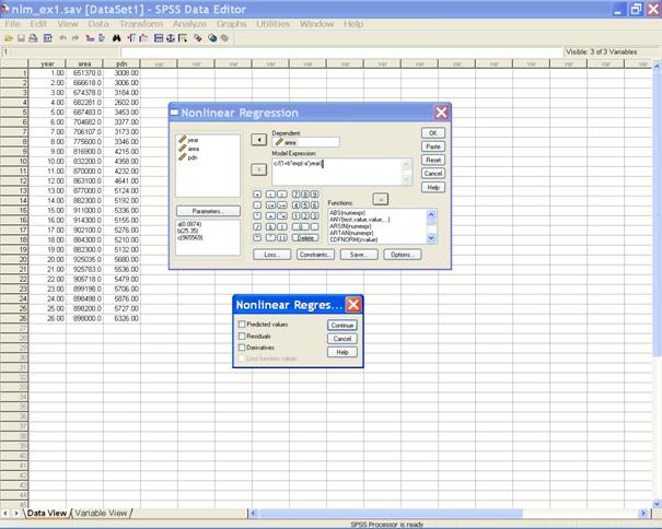
� In the Nonlinear Regression: Options dialog box select the desired estimation Method (Levenberg � Marquardt) and define the maximum iterations. � Click on Continue to return to the Nonlinear Regression dialog box. � Click on save tab.
� If one wants the predicted values and the residuals then in the dialog box check the appropriate options. � Click on Continue to return to the Nonlinear Regression dialog box.
� Click on OK to get the output. One
Step Ahead Forecasting (OSAF) for area under coconut Observed
value of 2005-06 is 898000 Predicted
value of 2005-06 is 925332.2 The
value of PCFE = 3.0436 Similarly
one may follows the above steps to fit the monomolecular and
gompertz models by changing the model expression
accordingly. After creating the data file one may use the following syntax to fit the nonlinear models for area under coconut. *Syntax
of logistic model for area under coconut. *
NonLinear Regression. MODEL
PROGRAM a=0.0874 b=25.35 c=965569. COMPUTE
PRED_ = c/(1+b*exp(-a*year)). NLR
area
/PRED PRED_
/SAVE PRED RESID
/CRITERIA ITER 50 SSCONVERGENCE 1E-10 PCON 1E-10 .
/*Observed
value of 2005-06 is 898000*/ /*Predicted
value of 2005-06 is 925332.2*/ /*The
value of PCFE = 3.0436*/ *Syntax
of Monomolecular model for area under coconut. *
NonLinear Regression. MODEL
PROGRAM a=.0874 b=25.35 c=965569 . COMPUTE
PRED_ = c-(c-b)*exp(-a*year). NLR
area
/PRED PRED_
/SAVE PRED RESID
/CRITERIA ITER 50 SSCONVERGENCE 1E-10 PCON 1E-10 . /*One
Step Ahead Forecasting (OSAF)*/ /*Observed
value of 2005-06 is 898000*/ /*Predicted
value of 2005-06 is 929878.3*/ /*The
value of PCFE = 3.549927*/ *Syntax
of Gompertz model for area under coconut. *
NonLinear Regression. MODEL
PROGRAM a=.108 b=.492 c=946477 . COMPUTE
PRED_ = c* exp(-b* exp(-a*year)). NLR
area
/PRED PRED_
/SAVE PRED RESID
/CRITERIA ITER 50 SSCONVERGENCE 1E-10 PCON 1E-10 . /*One
Step Ahead Forecasting (OSAF)*/ /*Observed
value of 2005-06 is 898000*/ /*Predicted
value of 2005-06 is 927556.8*/ /*The value of PCFE = 3.291402* After creating the data file one may use the following syntax to fit the nonlinear models for production of coconut. *Syntax
of logistic model for production of coconut. * NonLinear Regression. MODEL PROGRAM a=.01354 b=1.133 c=5876 . COMPUTE PRED_ = c/(1+b*exp(-a*year)). NLR pdn /PRED PRED_ /CRITERIA ITER 50 SSCONVERGENCE 1E-10 PCON 1E-10 . /*Observed
value of 2005-06 is 6326*/ /*Predicted
value of 2005-06 is 5898.58*/ /*The
value of PCFE = 6.76*/ *Syntax
of Monomolecular model for production of coconut. * NonLinear Regression. MODEL PROGRAM a=.01354 b=1.133 c=5876 . COMPUTE PRED_ = c-(c-b)*exp(-a*year). NLR pdn /PRED PRED_ /CRITERIA ITER 50 SSCONVERGENCE 1E-10 PCON 1E-10 . /*One
Step Ahead Forecasting (OSAF)*/ /*Observed
value of 2005-06 is 6326*/ /*Predicted
value of 2005-06 is 6021.69*/ /*The
value of PCFE = 4.81*/ *Syntax
of Gompertz model for production of coconut. * NonLinear Regression. MODEL PROGRAM a=.01354 b=1.133 c=5876 . COMPUTE PRED_ = c* exp(-b* exp(-a*year)). NLR pdn /PRED PRED_ /CRITERIA ITER 50 SSCONVERGENCE 1E-10 PCON 1E-10 . /*One
Step Ahead Forecasting (OSAF)*/ /*Observed
value of 2005-06 is 6326*/ /*Predicted
value of 2005-06 is 6781.4*/ /*The
value of PCFE = 7.198862*/ NOTE:
In SPSS, user has to calculate the OSAF value manually
Analysis Using SAS Analysis Using SPSS
Home Descriptive Statistics Tests of Significance Correlation and Regression Completely Randomised Design RCB Design Incomplete Block Design Resolvable Block Design Augmented Design Latin Square Design Factorial RCB Design Partially Confounded Design Factorial Experiment with Extra Treatments Split Plot Design Strip Plot Design Response Surface Design Cross Over Design Analysis of Covariance Diagnostics and Remedial Measures Principal Component Analysis Cluster Analysis Groups of Experiments Non-Linear Models
|
||||
| Descriptive Statistics | |||||
| Tests of Significance | |||||
| Correlation and Regression | |||||
| Completely Randomised Design | |||||
| RCB Design | |||||
| Incomplete Block Design | |||||
| Resolvable Block Design | |||||
| Augmented Design | |||||
| Latin Square Design | |||||
| Factorial RCB Design | |||||
| Partially Confounded Design | |||||
| Factorial Experiment with Extra Treatments | |||||
| Split Plot Design | |||||
| Strip Plot Design | |||||
| Response Surface Design | |||||
| Cross-Over Designs | |||||
| Analysis of Covariance | |||||
| Diagnostics and Remedial Measures | |||||
| Principal Component Analysis | |||||
| Cluster Analysis | |||||
| Groups of Experiments | |||||
| Non-Linear Models | |||||
| Contact Us | |||||
|
Other
Designed Experiments |
|||||
|
For
exposure on SAS, SPSS, Please
see Module
I of Electronic Book II: available at Design Resources Server (www.iasri.res.in/design) |
|||||


